Intro to A*
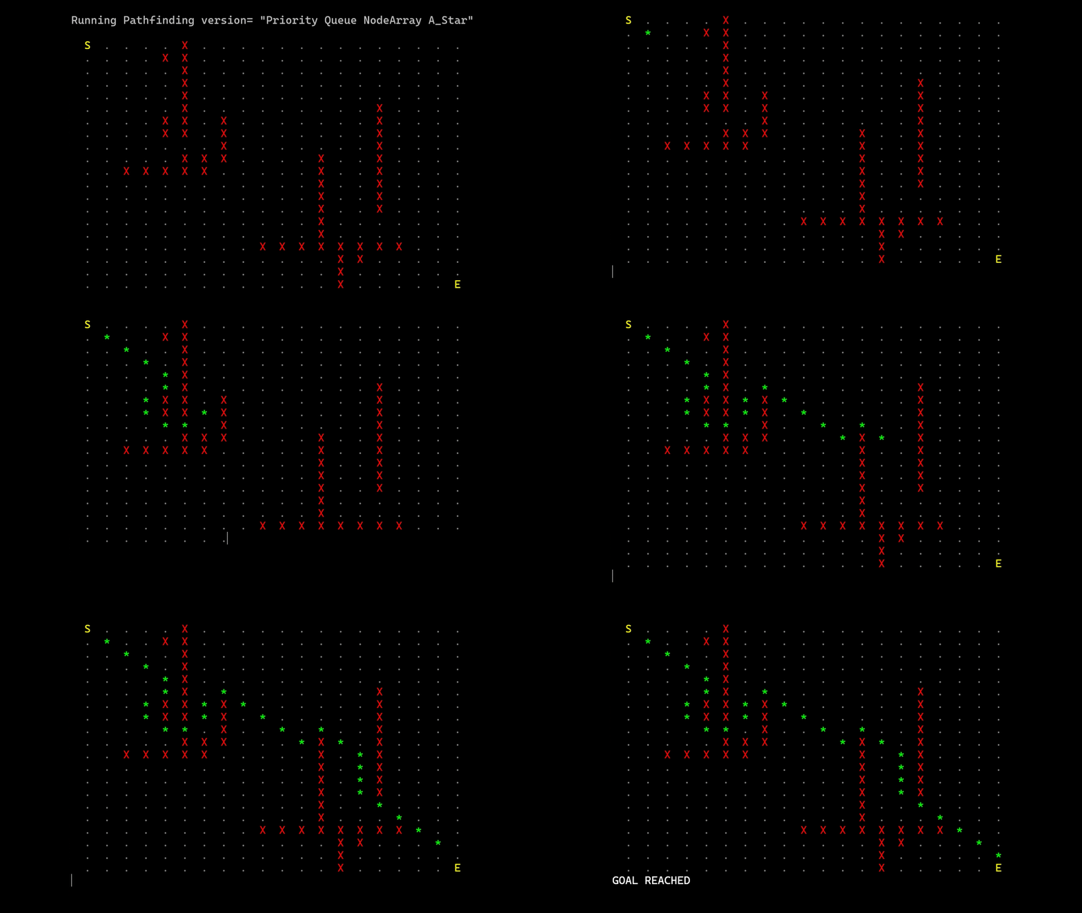
This is an implementation of the famous A* algorithm. This algorithm is primarly used in movement planning and solves the following problem:
Does a path exist between two points A and B? And if it does, which is the best?
In the general definition, this algorithm operates on a non negative weighted directed graph, searching for the optimal path guided by some cost function called heuristic. All the techniques used are described in the book AI for Games written by Ian Millington.
Profiler
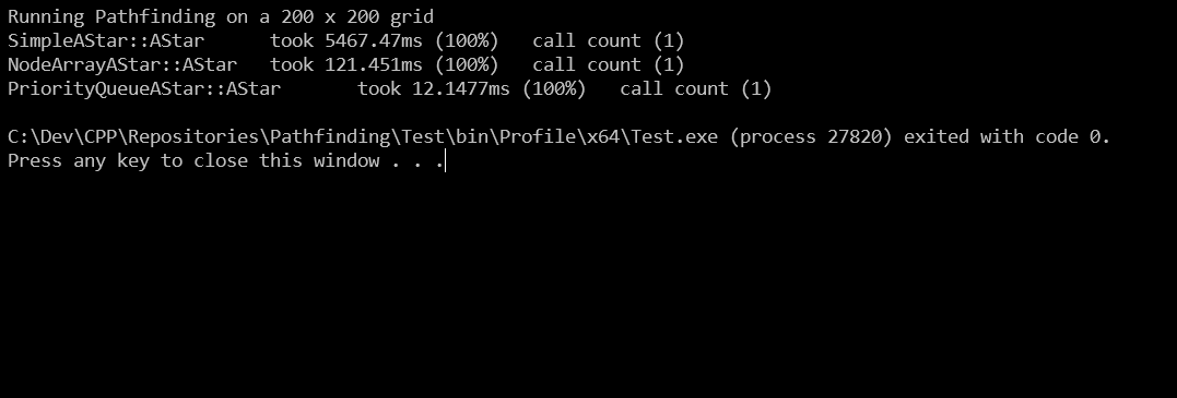
The algorithms performances has been tested through a scope profiling.
Such simple techique can be achieved putting timers, which lifecycle is tied with the start and end of a scope. I defined macros which can be put at the start of a scope, so the compiler can substitute them with profiling code or strip them out according to the application configuration.
Data related to the same function signature are accumulated. This can be used to determine the impact of a single function on the entire application.
Implementation
The algorithm uses an open list and a closed list of nodes.
The open list contains nodes that have not been visited yet. The closed list conatains all processed nodes. A node is moved in the open list as they are found at the end of connections. A node is moved in the closed list as they are processed during the iterations.
At each iteration, the node with the smallest estimated total cost is selected and processed. For the heuristic, I used the euclidean distance. This means it “thinks” that approaching to the target as the agent could fly is a good approximation. As Millington stated this is a good choice for outdoor maps, where there is a lot of movement freedom but performs badly in an indoor ones.
If there are no more open nodes and the goal was never reached, then a path won’t exists.
Of course, to retrieve the optimal path, the end node must be the one with the smallest cost so far (the true cost from the start node to the current one). This would remove any benefit to using A* instead of other algorithm like Dijkstra, so many implementations rely on the fact that a non-optimal path could be generated.
The resulting path is retrieved moving back from the end to the starting through all the selected nodes.

Node Array A*
One common techniques is to trade memory for performance. Instead of using different lists to store nodes, an array of all nodes can be preallocated. Each of these nodes, have a “category” (unvisited, open or closed). This can be expressed using a simple integer. This ereases the need of having a closed list. The open list is still needed since the node with the smallest estimated cost so far has to be chosen between the open nodes.
Heap Node Array A*
The complexity of finding the “best” current open node is O(n) (assuming an dynamic array data structure). A priority queue can be used to reduce this complexity to O(1) (insert and remove operations’ cost increases to O(nlog(n))).
